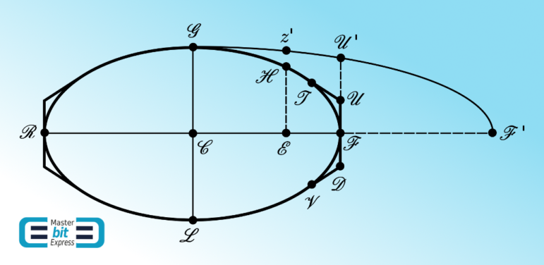
Dear User,

The subject of our previous post was the consideration of the Proposition XXXIV of Newton’s Philosophiae Naturalis Principia Mathematica. Sir Isaac Newton further considered the problem of the Proposition XXXIV, through the Scholium to this proposition in His Principia, by analyzing two important problems. The first of these problems of the Scholium is going to be subject of our consideration here – we are going to deal with the case of a frustum of cone through the analysis of Newton, having the objective of finding the best configuration to minimize the resistance of the frustum [of cone] against that same medium of inbounding particles as defined in the Proposition XXXIV. As we have pointed out in our previous post, the scope of the first problem of the Scholium, in spite of not being yet within a genuine resolution scope of Variational Calculus, is a scope that presents itself as inserted within a context of a variational necessity, having an important epistemological position – between the Proposition XXXIV and the second problem of the Scholium, the latter genuinely variational. This latter problem of the Scholium [to Proposition XXXIV] will be considered in details, not here yet, but as the subject of our next post. Hence, here through this post, we are going to proceed with the analysis of the first problem of the Scholium, following the same lines of reasoning took by Sir Isaac Newton in His Scholium to Proposition XXXIV of His Philosophiae Naturalis Principia Mathematica. As have been collected along the lines of consideration of our previous posts, we are going here to also find important concept, important to our journey – namely that the variational necessity presented by the first problem of the Scholium [to Proposition XXXIV], leading to the masterful resolution provided by Newton in the resolution of the second problem of the Scholium [to Proposition XXXIV], is conceptual gold to our forthcoming considerations, to our journey.

Path to Second Problem of Newton’s Scholium of 1685

Our previous post has considered the problem of determining which shape, spherical or cylindrical, is the best against the resistance of the fluid particles of a medium as defined by the Proposition XXXIV of Newton’s Principia. This latter investigation aims to discuss the cases considered as examples of resistance regarding a bow having blunt or hemispherical shapes. The analysis is the one with which is concerned the Proposition XXXIV of Newton’s Principia, a prelude to the more general case through which Sir Isaac Newton goes forward by reaching the resolutions which the Scholium to this latter proposition is provided to deal with. By considering the first problem of the Scholium, Sir Isaac Newton considers a frustum of a right-circular cone – finding the best shape given base and height, the case we are going to consider through this post.

The Figure 1 beneath depicts the geometrical situation regarding the cone. Figure 1 depicts the vertex \(\mathcal{Z}\) of the cone, its circular base \(\mathcal{BCDAB}\) having radius \(\mathcal{OB}\). The point \(\mathcal{P}\) equally divides the height \(\mathcal{OE}\) of the frustum. The frustum has a circular cap, being \(\mathcal{EF}\) the radius of this cap.

In our previous post, we have proposed an exercise. Recalling this exercise, we are going to provide the Figure 1 of our previous post again, our Figure 2 beneath with new inserted notations regarding the solution to that exercise – for purposes of the analysis with which we are going to proceed in a moment:

As we have seen in our previous post, the efficacy that correspondingly acts at point \(\mathcal{D}\) is a net effect that is exerted on the sphere along the \(\mathcal{FD}\) direction due to symmetry, being the force on the sphere distributed over the portion of line element \(dl\) so being proportional to:
\begin{equation}
\cos^{2}{\left(\mathcal{ADC}\right)}\cdot dl\cos{\left(\mathcal{ADC}\right)}=\cos^{3}{\left(\mathcal{ADC}\right)}\,dl.\tag{1}
\end{equation}

Due to symmetry, according to the Figure 2, the Eq. (1) is valid over all of the points over the \(2\pi y\) length of a ring around the \(x\) axis, so that an element of resistance reads:
\begin{equation}
dR=2\pi y\cdot\cos^{3}{\left(\mathcal{ADC}\right)}\,dl=2\pi y\cos^{2}{\left(\mathcal{ADC}\right)}\,dy,\tag{2}
\end{equation}

by virtue of:
\begin{equation}
dy=dl\cos{\left(\mathcal{ADC}\right)}.\tag{3}
\end{equation}

By integrating the elements of resistance given by the Eq. (2), between the initial and final ordinates, namely \(y_{i}\) and \(y_{f}\), we reach the Eq. (12) of our previous post: \begin{equation}
R=\oint dR=2\pi\int_{y_{i}}^{y_{f}}y\cos^{2}{\left(\mathcal{ADC}\right)}\,dy.\tag{4}
\end{equation}

Before going further to consider the case depicted by Figure 1, the case of the frustum we are going to analyze, it is important to consider the cases to which the Eq. (4) stands valid. First, the Eq. (4) is a result that stands from proportionality, i.e., the resistance it gives is constructed on an assumption of proportionality. But, being the units conveniently defined, this Eq. (4) seems to be able to be considered as the general equation for obtaining the resistance under the assumptions given by the Proposition XXXIV regarding the medium. This latter assumption does not suffice, since we are considering a symmetry of revolution. Hence, the Eq. (12) stands valid for surfaces having symmetry of revolution – and this Eq. (4) stands valid for that case of the frustum that is depicted by the Figure 1 and that we are going to consider – namely, that the Eq. (4) stands valid for considering the first problem of the Scholium to Proposition XXXIV. It is also important to grasp the meaning of the angle \(\mathcal{ADC}\) that enters the Eq. (12) prior to proceeding to a [general] case presenting symmetry of revolution. Considering the section presented by the Fig. 2, this is the angle between the normal to the circular section at a point \(\mathcal{D}\) and the \(x\) axis or, equivalently, the angle between the tangent to the circular section at \(\mathcal{D}\) and the \(y\) axis (the angle between \(dl\) and the vertical line – cf. the complementary depiction that has been provided through the Fig. 2) – correspondingly being the angle \(\mathcal{OBF}\) at point \(\mathcal{B}\) regarding the frustum depicted by the Figure 1.

To apply the Eq. (4) to the case of the frustum of cone, as depicted by the Figure 1, it is necessary to obtain the resistance of the lateral surface of the frustum generated by the revolution of the curve \(\mathcal{BF}\) around the \(\mathcal{OE}\) axis. For this purpose, we define the \(x0y\) as being \(\mathcal{ZOB}\), so that to reach the state of affairs of the Figure 3 beneath regarding the Figure 1:

Hence, from the Eq. (4) and from the Figure 3, we obtain the resistance of the lateral surface of the frustum generated by the revolution of the curve \(\mathcal{BF}\) around the \(\mathcal{OE}\) axis:
\begin{equation}
R_{\mathcal{BF}}=2\pi\int_{\mathcal{EF}}^{\mathcal{OB}}y\cos^{2}{\mathcal{\left(OBF\right)}}\,dy.\tag{5}
\end{equation}

Also, it is important to observe that the angle \(\mathcal{OBF}\) is constant considering the given cone, since:
\begin{eqnarray}
\cot{\mathcal{\left(OBF\right)}}&=&\dfrac{\mathcal{OB}}{\mathcal{OZ}}\Rightarrow\nonumber\\
\mathcal{OBF}&=&\cot^{-1}{\left(\dfrac{\mathcal{OB}}{\mathcal{OZ}}\right)}=\text{const.}\tag{6}
\end{eqnarray}

By virtue of Eqs. (5) and (6), we reach:
\begin{eqnarray}
R_{\mathcal{BF}}&=&2\pi\cos^{2}{\left(\mathcal{OBF}\right)}\int_{\mathcal{EF}}^{\mathcal{OB}}y\,dy\,\,\Rightarrow\nonumber\\
R_{\mathcal{BF}}&=&2\pi\cos^{2}{\left(\mathcal{OBF}\right)}\left.\dfrac{y^{2}}{2}\,\right|_{\mathcal{EF}}^{\mathcal{OB}}\nonumber\\
&=&\pi\cos^{2}{\left(\mathcal{OBF}\right)}\left[\left(\mathcal{OB}\right)^{2}-\left(\mathcal{EF}\right)^{2}\right].\tag{7}
\end{eqnarray}

The resistance on the frontal cap of the frustum is obtained from the Eq. (4) with \(\mathcal{EFE}=0\Rightarrow\cos{\left(\mathcal{EFE}\right)}=1=\text{const.}\), from which:
\begin{eqnarray}
R_{\mathcal{FE}}&=&2\pi\cos^{2}{\left(\mathcal{EFE}\right)}\int_{0}^{\mathcal{EF}}y\,dy\,\,\Rightarrow\nonumber\\
R_{\mathcal{FE}}&=&2\pi\left.\dfrac{y^{2}}{2}\,\right|_{0}^{\mathcal{EF}}\nonumber\\
&=&\pi\left(\mathcal{EF}\right)^{2}.\tag{8}
\end{eqnarray}

Now, from the Eqs. (7) and (8), we obtain the total resistance over the frustum:
\begin{eqnarray}
R_{\mathcal{BFE}}&=&\oint_{\mathcal{BFE}}dR=R_{\mathcal{BF}}+R_{\mathcal{FE}}\nonumber\\
&=&\pi\cos^{2}{\left(\mathcal{OBF}\right)}\left[\left(\mathcal{OB}\right)^{2}-\left(\mathcal{EF}\right)^{2}\right]+\pi\left(\mathcal{EF}\right)^{2}\nonumber\\
&=&\pi\left[\left(\mathcal{OB}\right)^{2}\cos^{2}{\left(\mathcal{OBF}\right)}+\left(\mathcal{EF}\right)^{2}\sin^{2}{\left(\mathcal{OBF}\right)}\right]\nonumber\tag{9}
\end{eqnarray}

where we have used the identity \(1-\cos^{2}{\left(\mathcal{OBF}\right)}=\sin^{2}{\left(\mathcal{OBF}\right)}\). From the Figure 1, we infer the following trigonometric relations:
\begin{eqnarray}
\sin{\mathcal{\left(OBF\right)}}&=&\dfrac{\mathcal{OZ}}{\mathcal{BZ}}=\dfrac{\mathcal{OE}+\mathcal{EZ}}{\sqrt{\left(\mathcal{OB}\right)^{2}+\left(\mathcal{OZ}\right)^{2}}}\nonumber\\
&=&\dfrac{\mathcal{OE}+\mathcal{EZ}}{\sqrt{\left(\mathcal{OB}\right)^{2}+\left(\mathcal{OE}+\mathcal{EZ}\right)^{2}}}\Rightarrow\nonumber\\
\sin^{2}{\mathcal{\left(OBF\right)}}&=&\dfrac{\left(\mathcal{OE}+\mathcal{EZ}\right)^{2}}{\left(\mathcal{OB}\right)^{2}+\left(\mathcal{OE}+\mathcal{EZ}\right)^{2}}\tag{10}
\end{eqnarray}

\begin{eqnarray}
\cos{\mathcal{\left(OBF\right)}}&=&\dfrac{\mathcal{OB}}{\mathcal{BZ}}=\dfrac{\mathcal{OB}}{\sqrt{\left(\mathcal{OB}\right)^{2}+\left(\mathcal{OZ}\right)^{2}}}\nonumber\\
&=&\dfrac{\mathcal{OB}}{\sqrt{\left(\mathcal{OB}\right)^{2}+\left(\mathcal{OE}+\mathcal{EZ}\right)^{2}}}\Rightarrow\nonumber\\
\cos^{2}{\mathcal{\left(OBF\right)}}&=&\dfrac{\left(\mathcal{OB}\right)^{2}}{\left(\mathcal{OB}\right)^{2}+\left(\mathcal{OE}+\mathcal{EZ}\right)^{2}}\tag{11}
\end{eqnarray}

The substitution of the results from Eqs. (10) and (11) within the right-hand side of the Eq. (9) gives:
\begin{equation}
R_{\mathcal{BFE}}=\pi\dfrac{\left(\mathcal{OB}\right)^{4}+\left(\mathcal{EF}\right)^{2}\left(\mathcal{OE}+\mathcal{EZ}\right)^{2}}{\left(\mathcal{OB}\right)^{2}+\left(\mathcal{OE}+\mathcal{EZ}\right)^{2}}.\tag{12}
\end{equation}

By reading the following trigonometric relation from the Figure 1 regarding the triangles \(\mathcal{OBZ}\) and \(\mathcal{EFZ}\):
\begin{equation}
\cot{\left(\mathcal{OBF}\right)}=\dfrac{\mathcal{OB}}{\mathcal{OZ}}=\dfrac{\mathcal{EF}}{\mathcal{EZ}},\tag{13}
\end{equation}

we reach the relation:
\begin{eqnarray}
\dfrac{\mathcal{EZ}}{\mathcal{OZ}}=\dfrac{\mathcal{EF}}{\mathcal{OB}}&=&\dfrac{\mathcal{EZ}}{\mathcal{OE}+\mathcal{EZ}}\Rightarrow\nonumber\\
\left(\mathcal{EF}\right)\left(\mathcal{OE}+\mathcal{EZ}\right)&=&\left(\mathcal{EZ}\right)\left(\mathcal{OB}\right)\nonumber\\
&\Rightarrow&\nonumber\\
\left(\mathcal{EF}\right)^{2}\left(\mathcal{OE}+\mathcal{EZ}\right)^{2}&=&\left(\mathcal{EZ}\right)^{2}\left(\mathcal{OB}\right)^{2},\tag{14}
\end{eqnarray}

which, substituted within the right-hand side of the Eq. (12), provides:
\begin{equation}
\dfrac{R_{\mathcal{BFE}}}{\pi\left(\mathcal{OB}\right)^{2}}=\dfrac{\left(\mathcal{OB}\right)^{2}+\left(\mathcal{EZ}\right)^{2}}{\left(\mathcal{OB}\right)^{2}+\left(\mathcal{OE}+\mathcal{EZ}\right)^{2}}.\tag{15}
\end{equation}

By requiring that:
\begin{equation}
\dfrac{d}{d\left(\mathcal{EZ}\right)}\left(\dfrac{R_{\mathcal{BFE}}}{\pi\left(\mathcal{OB}\right)^{2}}\right)=\dfrac{1}{\pi\left(\mathcal{OB}\right)^{2}}\dfrac{d}{d\left(\mathcal{EZ}\right)}R_{\mathcal{BFE}}=0,\tag{16}
\end{equation}

the condition:
\begin{equation}
\dfrac{d}{d\left(\mathcal{EZ}\right)}R_{\mathcal{BFE}}=0\tag{17}
\end{equation}

also follows required, which is necessary if the Eq. (12) presents a minimum at some value of its independent variable \(\mathcal{EZ}\). At this point, we are going to propose the following exercise:

• By obtaining the derivative of the right-hand side of the Eq. (15) and applying the condition given by the Eq. (17), show that the following condition follows required:

\begin{equation}
\left(\mathcal{EZ}\right)^{2}+\left(\mathcal{OE}\right)\left(\mathcal{EZ}\right)-\left(\mathcal{OB}\right)^{2}=0.\tag{18}
\end{equation}

By solving the Eq. (18), the configuration that provides the minimum resistance to the frustum of cone against the inbounding colliding particles of the medium according to the scenario following from the proposition and from the first problem of the Newton’s Scholium to this proposition (Proposition XXXIV) of His Principia is the one to which:
\begin{equation}
\mathcal{EZ}=-\dfrac{\mathcal{OE}}{2}+\sqrt{\,\left(\dfrac{\mathcal{OE}}{2}\right)^{2}+\left(\mathcal{OB}\right)^{2}\,}\,.\tag{19}
\end{equation}

This result suffices to understand why Sir Isaac Newton asserts in the Scholium, namely to Prop. XXXV Theor. XXVIII of the second book of the published Principia – afterwards advanced to be Proposition XXXIV in the second edition, that: biseca altitudine \(\mathcal{OE}\) in \(\mathcal{P}\) et produc \(\mathcal{OP}\) ad \(\mathcal{Z}\) ut sit \(\mathcal{PZ}\) aequalis \(\mathcal{PB}\), et erit \(\mathcal{Z}\) vertex coni cujus frustum quaeritur.

Sir Isaac Newton is saying that, to find the frustum of cone that exerts the least resistance against the defined medium, one bisects the height \(\mathcal{OE}\) in \(\mathcal{P}\), to produce \(\mathcal{OP}\) along \(\mathcal{OE}\) and by reaching a point \(\mathcal{Z}\) by continuation along the same line such that \(\mathcal{PZ}\) is equal to \(\mathcal{PB}\) – so that with then \(\mathcal{Z}\) being the vertex of the cone whose frustum is sought. This is so, since, from the construction of the Figure 1, \(\mathcal{OP}=\mathcal{OE}/2\), which, from the Eq. (19), gives:
\begin{eqnarray}
\mathcal{OZ}&=&\mathcal{OE}+\mathcal{EZ}=\mathcal{OE}-\dfrac{\mathcal{OE}}{2}+\sqrt{\,\left(\dfrac{\mathcal{OE}}{2}\right)^{2}+\left(\mathcal{OB}\right)^{2}\,}\nonumber\\
&=&\dfrac{\mathcal{OE}}{2}+\sqrt{\,\left(\dfrac{\mathcal{OE}}{2}\right)^{2}+\left(\mathcal{OB}\right)^{2}\,}\nonumber\\
&=&\dfrac{\mathcal{OE}}{2}+\sqrt{\,\left(\mathcal{OP}\right)^{2}+\left(\mathcal{OB}\right)^{2}\,}=\mathcal{OP}+\mathcal{PB},\tag{20}
\end{eqnarray}

where we have used the relation \(\left(\mathcal{PB}\right)^{2}=\left(\mathcal{OP}\right)^{2}+\left(\mathcal{OB}\right)^{2}\) also from the construction of the Figure 1. Now from Eq. (20) and Figure 1:
\begin{equation}
\mathcal{PZ}=\mathcal{OZ}-\mathcal{OP}=\mathcal{OP}+\mathcal{PB}-\mathcal{OP}=\mathcal{PB}.\tag{21}
\end{equation}

So that, we have constructed the best frustum of cone that minimizes the resistance against the medium according to the Proposition XXXIV of Newton’s Principia. Sir Isaac Newton goes further, by considering then a section having elliptical nature as depicted by the Figure beneath:

Newton engages through a discussion regarding a more general form of solid of revolution, starting with the case depicted by the Figure 4 – to analyze its resistance against that same medium composed by the inbounding colliding particles previously defined in the Proposition XXXIV of His Principia. For purposes of analyzing the Figure 4, let the frustum height be zero, i.e., let \(\mathcal{OE}\to 0\). From Eq. (20), this implies that \(\mathcal{OZ}\to\mathcal{OB}\). The consequence is that the angles \(\mathcal{BZO}=\mathcal{OZD}\) turn out to be \(\pi/4\). Hence, the lines \(\mathcal{BZ}\) and \(\mathcal{ZD}\) will contain obtuse angles of \(3\pi/4\) with a vertical line parallel to \(\mathcal{OB}\) passing through the \(\mathcal{Z}\) point. Now, we translate this latter scenario to the Figure 4. Sir Isaac Newton asserts that: Unde obiter, cum angulus \(\mathcal{BZD}\) [in Figure 1] semper sit acutus, consequens est quod si solidum \(\mathcal{RGFLR}\) [in Figure 4] convolutione figurae Ellipticae vel Ovalis \(\mathcal{RGFLR}\) circa axem \(\mathcal{RF}\) generetur, et tangatur figura generans a rectis tribus \(\mathcal{TU}\), \(\mathcal{UD}\), \(\mathcal{DV}\) in punctis \(\mathcal{T}\), \(\mathcal{F}\) et \(\mathcal{V}\) ea lege ut \(\mathcal{UD}\) sit perpendicularis ad axem in puncto contactus \(\mathcal{F}\) et \(\mathcal{TU}\), \(\mathcal{DV}\) cum \(\mathcal{UD}\) contineant angulos \(\mathcal{TUF}\), \(\mathcal{FDV}\) graduum 135: solidum quod convolutione figurae \(\mathcal{RGTUFDVLR}\) circa axem eundem generetur minus resistetur quam solidum prius si modo utrumq secundum plagam axis sui \(\mathcal{RF}\) progrediatur, & utriusq terminus \(\mathcal{F}\) praecedat. Quam quidem Propositionem in construendis navibus non inutilem futuram esse censeo.

Sir Isaac Newton is saying that the solid generated by the revolution of the \(\mathcal{RGFLR}\) oval around the \(\mathcal{RF}\) axis is going to present more resistance than the solid generated by the revolution of the \(\mathcal{RGTUFDVLR}\) touched oval around the \(\mathcal{RF}\) axis, this latter figure constructed under the requirements of angle regarding the \(\mathcal{BZ}\) and \(\mathcal{ZD}\) lines as delineated above, in the sense that the frustum of cone \(\mathcal{TUDV}\) is going to act against less resistance than will the \(\mathcal{TFV}\) portion of the oval. This assertion needs to be proved, but Sir Isaac Newton provided no indication over how He achieved the assertion. To understand this previous assertion Sir Isaac Newton gave to us, under a mathematical reasoning, we are going to follow the remarks that have been given by D.T. Whiteside in The Mathematical Papers of Isaac Newton, Volume VI, page 462, footnote 22.

For analyzing the previous assertion of Newton under the remarks of D.T. Whiteside, we are going to use the Figure 5 beneath. As we have previously commented, regarding the Figure 1, when the height \(\mathcal{OE}\) of the frustum \(\mathcal{BFLDB}\) of the cone \(\mathcal{BZDB}\) tends to be infinitesimal: \(\mathcal{BP}\to\mathcal{BO}\), \(\mathcal{PZ}\to\mathcal{OZ}\) and \(\mathcal{BF}\) becomes inclined at \(\pi/4\) to the \(\mathcal{OE}\) axis. In the Figure 5, let us consider the tangent \(\mathcal{TU}\) inclined at \(\pi/4\) to the axis \(\mathcal{CF}\) and containing the arc \(\mathcal{TF}\) so that the points \(\mathcal{H}\) and \(h\) pertaining to the arc \(\mathcal{TF}\) are taken to be two indefinitely close points in the arc entirely contained by the tangent \(\mathcal{TU}\) and the vertical lines \(\mathcal{FU}\) and \(\mathcal{Tt}\) at the end-points \(\mathcal{F}\) and \(\mathcal{T}\). We then respectively construct the ordinates \(\mathcal{EH}\) and \(eh\) of the points \(\mathcal{H}\) and \(h\). The line \(hs\) is constructed starting from point \(h\), parallel to the tangent \(\mathcal{TU}\), until reaching the continuation of \(\mathcal{EH}\) at \(s\).

Observing that, in Figure 5, the infinitesimal frustum of cone \(\mathcal{E}she\mathcal{E}\) is under a configuration having its lateral surface \(sh\) under an angle that provides minimum resistance against the medium, a configuration that we have reached above by requiring that, to the frustum height [\(\mathcal{OE}\) in Figure 1], \(\mathcal{OE}=e\mathcal{E}\to 0\), it follows that the resistance against \(\mathcal{EH}h\) is greater than the resistance against \(\mathcal{E}sh\). Ignoring the common surface \(\mathcal{EH}\) over which the resistance is the same in both the cases, it follows that the resistance against \(\mathcal{H}h\) is greater than the resistance against \(\mathcal{H}sh\). Hence, we conclude that the element of surface that is generated by rotating \(\mathcal{H}h\) around the \(\mathcal{CF}\) axis will encounter a resistance from the medium against it that is greater than the resistance from the same medium the element of surface that is generated by rotating \(\mathcal{H}sh\) around the \(\mathcal{CF}\) axis will encounter against it. Hence, having the resolution by touching the oval so that to permit the construction of a portion of the oval \(\mathcal{TF}\) beneath the optimum frustum lateral generating line \(\mathcal{TU}\), each infinitesimal portion along the arc \(\mathcal{TF}\) will resist more than the locally constructed and generated surface of optimal frustum, such that then existing \(sq\) and \(\mathcal{H}r\) that fall projected perpendicularly to \(eh\) along the \(\mathcal{CF}\) direction. Defining the axes \(0x\) and \(0y\) respectively along the \(\mathcal{F}t\) and \(t\mathcal{T}\) axes, one reads from the geometry as depicted by the Figure 5:
\begin{eqnarray}
dx=qh=qs=e\mathcal{E},\tag{22}\\
dy=rh=eh-\mathcal{EH},\tag{23}
\end{eqnarray}

where we have used the fact: the angle \(hsq\) is \(\pi/4\). Now, we locally use the Eq. (4) to obtain the resistance of the surface that is generated by rotating \(\mathcal{H}sh\) around the \(\mathcal{CF}\) axis. For the portion due to \(\mathcal{H}s\), the angle \(\mathcal{H}s\mathcal{H}\) is \(0\), and the Eq. (2) then turns out to locally give:
\begin{eqnarray}
dR_{\mathcal{H}s}&=&2\pi\,\mathcal{EH}\,\cos^{2}{\left(0\right)}\,\mathcal{H}s=2\pi\,\mathcal{EH}\,(rh-qh)\nonumber\\
&=&2\pi\,\mathcal{EH}\,(dy-dx),\tag{24}
\end{eqnarray}

where we have used the Eqs. (22) and (23). For the portion due to \(sh\), the angle \(qhs\) is \(\pi/4\), and the Eq. (2) then turns out to locally give:
\begin{eqnarray}
dR_{sh}&=&2\pi\,\mathcal{E}s\,\cos^{2}{\left(\pi/4\right)}\,qh\nonumber\\
&=&\pi\,\left(\mathcal{EH}+\mathcal{H}s\right)\,qh\nonumber\\
&=&\pi\,\mathcal{EH}\,qh+\pi\,\mathcal{H}s\,qh\nonumber\\
&=&\pi\,\mathcal{EH}\,qh=\pi\,\mathcal{EH}\,dx\tag{25}
\end{eqnarray}

where we have used the Eq. (22). Hence. by virtue of the Eqs. (24) and (25), the resistance of the surface that is generated by rotating \(\mathcal{H}sh\) around the \(\mathcal{CF}\) axis is:
\begin{eqnarray}
dR_{\mathcal{H}sh}&=&2\pi\,\mathcal{EH}\,(dy-dx)+\pi\,\mathcal{EH}\,dx\nonumber\\
&=&2\pi\,\mathcal{EH}\,dy-\pi\,\mathcal{EH}\,dx\nonumber\\
&=&2\pi\,y\,dy-\pi\,y\,dx=\pi\left(2y\,dy-y\,dx\right).\tag{26}
\end{eqnarray}

Henceforth, the resistance \(R_{\mathcal{FT}}\) of the solid that is generated by rotating the arc \(\mathcal{FT}\) around the \(\mathcal{CF}\) axis is such that:
\begin{eqnarray}
R_{\mathcal{FT}}&>&\pi\int_{0}^{t\mathcal{T}}2y\,dy-\pi\int_{0}^{\mathcal{F}t}y\,dx\nonumber\\
&=&\pi\int_{0}^{\mathcal{FU}}2y\,dy+\pi\int_{\mathcal{FU}}^{t\mathcal{T} }2y\,dy-\pi\int_{0}^{\mathcal{F}t}y\,dx\nonumber\\
&>&\pi\int_{\mathcal{FU}}^{t\mathcal{T} }2y\,dy-\pi\int_{0}^{\mathcal{F}t}y\,dx\nonumber\\
&=&\left.\pi y^{2}\,\right|_{\mathcal{FU}}^{t\mathcal{T}}-\pi\int_{0}^{\mathcal{F}t}y\,dx\nonumber\\
&=&\pi\left[\left(t\mathcal{T}\right)^{2}-\left(\mathcal{FU}\right)^{2}\right]-\pi\int_{0}^{\mathcal{F}t}y\,dx\nonumber\\
&=&2\dfrac{\pi}{2}\left[\left(t\mathcal{T}\right)^{2}-\left(\mathcal{FU}\right)^{2}\right]-\pi\int_{0}^{\mathcal{F}t}y\,dx\tag{27}
\end{eqnarray}

But, we also have that:
\begin{eqnarray}
\left[\left(t\mathcal{T}\right)^{2}-\left(\mathcal{FU}\right)^{2}\right]&=&\left(t\mathcal{T}+\mathcal{FU}\right)\left(t\mathcal{T}-\mathcal{FU}\right)\nonumber\\
&=&\left(t\mathcal{T}+\mathcal{FU}\right)\,\mathcal{F}t,\tag{28}
\end{eqnarray}

since the angle \(t\mathcal{TU}\) is \(\pi/4\). But, the quantity:
\begin{equation}
\dfrac{1}{2}\left(t\mathcal{T}+\mathcal{FU}\right)\,\mathcal{F}t\tag{29}
\end{equation}

is the area of the trapezoid \(t\mathcal{FUT}t\), which is greater than the area of the curve \(\mathcal{FT}\), so that the following inequality holds:
\begin{eqnarray}
\int_{0}^{\mathcal{F}t}y\,dx&<&\dfrac{1}{2}\left(t\mathcal{T}+\mathcal{FU}\right)\,\mathcal{F}t\Rightarrow\nonumber\\
\pi\int_{0}^{\mathcal{F}t}y\,dx&<&\dfrac{\pi}{2}\left(t\mathcal{T}+\mathcal{FU}\right)\,\mathcal{F}t\Rightarrow\nonumber\\ -\pi\int_{0}^{\mathcal{F}t}y\,dx&>&-\dfrac{\pi}{2}\left(t\mathcal{T}+\mathcal{FU}\right)\,\mathcal{F}t.\tag{30}
\end{eqnarray}

Now, using the Eq. (28) to rewrite the Eq. (27):
\begin{equation}
R_{\mathcal{FT}}>2\dfrac{\pi}{2}\left(t\mathcal{T}+\mathcal{FU}\right)\,\mathcal{F}t-\pi\int_{0}^{\mathcal{F}t}y\,dx,\tag{31}
\end{equation}

we reach, by virtue of the Eq. (30)
\begin{equation}
R_{\mathcal{FT}}>2\dfrac{\pi}{2}\left(t\mathcal{T}+\mathcal{FU}\right)\,\mathcal{F}t-\dfrac{\pi}{2}\left(t\mathcal{T}+\mathcal{FU}\right)\,\mathcal{F}t,\tag{32}
\end{equation}

i.e.:
\begin{equation}
R_{\mathcal{FT}}>\dfrac{\pi}{2}\left(t\mathcal{T}+\mathcal{FU}\right)\,\mathcal{F}t,\tag{33}
\end{equation}

or, using the Eq. (28), we finally reach the assertion Sir Isaac Newton gave but with no indication about how He reached it:
\begin{equation}
R_{\mathcal{FT}}>\dfrac{\pi}{2}\left[\left(t\mathcal{T}\right)^{2}-\left(\mathcal{FU}\right)^{2}\right].\tag{34}
\end{equation}

By comparing the right-hand side of Eq. (34) with Eq. (7), we see that the right-hand side of Eq. (34) is the resistance of a frustum of cone having \(\mathcal{OBF}=\pi/4\) angle in Figure 1. The Eq. (34) is exactly the assertion of Newton that says that the total resistance \(R_{\mathcal{FT}}\) the solid that is generated by the revolution of \(\mathcal{FT}\) in Figure 4 around the \(\mathcal{CF}\) axis exerts against the medium is greater than the resistance a frustum that is generated by the revolution of \(\mathcal{TUF}\) in Figure 4 around the \(\mathcal{CF}\) axis exerts against the medium.

We have reached the first problem of the Scholium and the initial considerations to the analysis that goes further to the second problem. The latter assertion of Newton is not an assertion about the best shape yet. The general problem regards the second problem of the Scholium. As an exercise:

• Consider the Figure beneath. Based on an analysis of this Figure, give a list of reasons to improve the arguments of Sir Isaac Newton based on Figure 4.

Next post, we will consider the second problem of the Scholium – Newton’s magistral solution to the second problem and the birth of a new mathematical field.

See You there. And all the best, indeed,

MasterBitExpress Bitcoin Wallet
Development